Chapter 6 Continuous Probability Distributions

In order to determine the probability of acceptance the individual probabilities for 0 and 1 defectives are summed. Additionally the probability of the whole sample space should equal one as it contains all outcomes P outcomes in total 18.

Continuous Probability Distributions Basic Introduction Youtube

A probability distribution specifies the relative likelihoods of all possible outcomes.

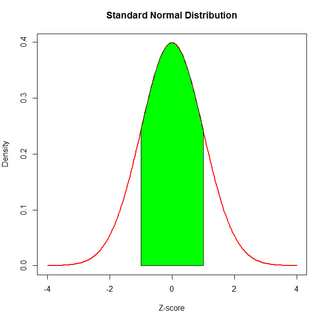
. For some positive value of Z the probability that a standard normal variable is between 0 and Z is 03770. The times of commercial flights between Atlanta and Los Angeles are 467 hours 513 hours and so on. For discrete random variables the PMF is a function from Sto the interval 01 that associates a probability with each x2S ie fx PX x.

If we discretize X by measuring depth to the nearest meter then possible values are nonnegative integers less. 32 - Probability trees. Can assume an infinite number of values within a given range.

For example in Chapter 4 the number of successes in a Binomial experiment was explored and in Chapter 5 several popular distributions for a continuous random variable were considered. P x x P Xx For all x belongs to the range of X. C It is a discrete probability distribution.

54 Sampling Distribution of the Mean. Would you take this bet. B About 23 of the observations fall within 1 standard deviation from the mean.

Continuous Improvement Toolkit. Google Slides LaTeX variants available. 6 Continuous Random Variables A nondiscrete random variable X is said to be absolutely continuous or simply continuous if its distribution func-tion may be represented as 7 where the function fx has the properties 1.

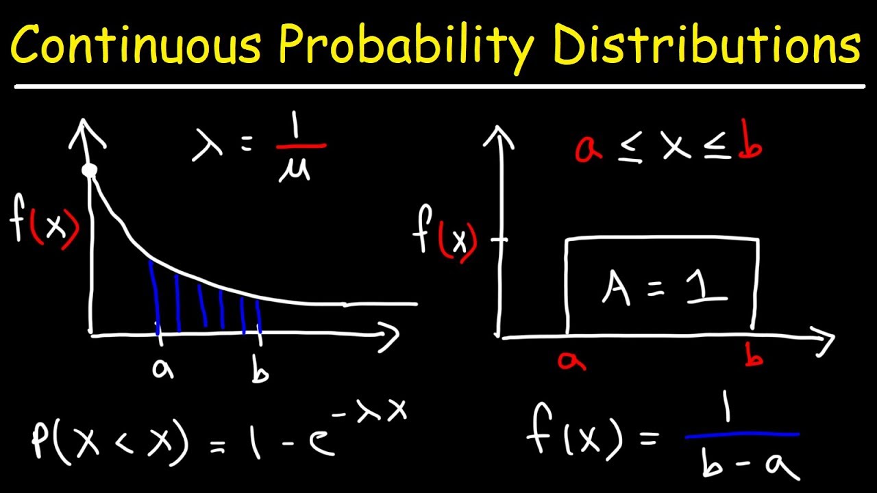
We also introduce the q prefix here which indicates the inverse of the cdf function. The probability distribution of a continuous random variable X is an assignment of probabilities to intervals of decimal numbers using a function f x called a density function The function f x such that probabilities of a continuous random variable X are areas of regions under the graph of y f x in the following way. The Probability Mass Function PMF is also called a probability function or frequency function which characterizes the distribution of a discrete random variable.

Go to Probability Distributions. 62 Joint Probability Mass Function. It may be any set.

In the context of probability theory we use set notation to specify compound events. LaTeX slides for full. Useful tool for conditional probability.

P 1 or less P0 P1 0358. Continuous Probability Distributions 188 Figure 612. The value of Z is a 018 b 081 c 116 d 1.

Uniform Distribution with P5 x 10 How would you find this probability. 441 Computations with normal random variables. For any event of a random experiment we can find its corresponding probability.

Let X be a discrete random variable of a function then the probability mass function of a random variable X is given by. Sampling From a Box. It follows from the.

In Chapter 1 an axiomatic framework is presented while in Chapter 2 the important concept of a random vari-able is introduced. 6 Joint Probability Distributions. For example if time is infinite.

Chapter 2 Compound Probability. The root name for these functions is norm and as with other distributions the prefixes d p and r specify the pdf cdf or random sampling. Some examples of continuous probability distributions are normal.

The height weight age of a person the distance between two cities etc. For example we can represent the event roll an even number by the set 2 4 6. 4 Probability Distributions for Continuous Variables Suppose the variable X of interest is the depth of a lake at a randomly chosen point on the surface.

A probability distribution is a mathematical description of the probabilities of events subsets of the sample spaceThe sample space often denoted by is the set of all possible outcomes of a random phenomenon being observed. Core concepts explained in detail. R has built-in functions for working with normal distributions and normal random variables.

The values of random variables. Statistics Using Technology 2nd Edition by Kathryn Kozak. Notice that the shape of the shaded area is a rectangle and the area of a rectangle is length times width.

The random variable is the time in hours and is measured on a continuous scale of time. A set broadly defined is a collection of objects. 31 - Defining probability.

Probability distributions are of two types which are continuous probability distributions and discrete probability distributions. The posterior probability is a type of conditional probability that results from updating the prior probability with information summarized by the likelihood through an application of Bayes theorem. 52 The Uniform Distribution.

The length is 1055 and the. Chapter 3 Probability Distributions. Chapter 4 Frequentist Inference.

Videos for some sections. Chapters 1 and 2 deal with basic ideas of probability theory. From an epistemological perspective the posterior probability contains everything there is to know about an uncertain proposition such as a scientific hypothesis or parameter.

Slides 3 - Probability. Chi-Square and ANOVA Tests. Schaums Outline of Probability and Statistics CHAPTER 2 Random Variables and Probability Distributions 35.

A set of real numbers a set of vectors a set of arbitrary non-numerical values etcFor example the sample space of a coin flip would. BASIC PROBABILITY THEORY 3 Probabilities of unions of disjoint events should equal the sum of the individual probabilities. A paperback bound copy of.

Statistics Using Technology 2nd Edition by Kathryn Kozak. D Its parameters are the mean and standard deviation 3. It is measured on a continuous interval or ratio scale.

Slides for each section. 53 Binomial Probabilities and the Normal Curve. Discrete and Continuous.

Let M the maximum depth in meters so that any number in the interval 0 M is a possible value of X. It is noted that the probability function. When sampling we commonly want to accept a batch if there are say 1 or less defective in the sample and reject it if there are 2 or more.

A continuous probability distribution contains an infinite number of values. In Chapters 4 and 5 the focus was on probability distributions for a single random variable. Central Limit Theorem.

Continuous random variables will also create continuous probability distributions hence their graphs will also be continuous. For this reason it is important to. For different values of the random variable we can find its respective probability.

Are some of the continuous random variables. A Baseball Spinner Game. Frequentist inference is the process of determining properties of an underlying distribution via the observation of data.

The probability that X assumes a value in the interval a b is. Section 261 gives a simple derivation of the joint distribution of the sample mean and sample variance of a normal data sample. Calculus says that the probability is the area under the curve.

Thinking through probability and risk. As another reminder a probability distribution has an associated function f that is referred to as a probability mass function PMF or probability distribution function PDF. This chapter discusses further concepts that lie at the core of probability theory.

Continuous Probability Distribution An Overview Sciencedirect Topics

Continuous Probability Distributions Env710 Statistics Review Website

Continuous Probability Distributions Env710 Statistics Review Website

Continuous Probability Distributions Env710 Statistics Review Website